Blog · May 19, 2026
DP, Monte Carlo, and TD: Three Ways to Solve the Bellman Equation
The throughline: The value of where I am is the reward I just got, plus a discounted value of where I’ll land next. Last post we wrote that equation. This post we solve it three different ways.
1. The intuition
In MDPs & Bellman we derived the Bellman equation, the recursive statement that connects a state’s value to its successors. But having an equation isn’t the same as having a number. How do we actually compute ?
Three families of algorithms, three different assumptions:
| Method | What it needs | When it updates |
|---|---|---|
| Dynamic Programming | The full model | Every state, every sweep |
| Monte Carlo | Complete episodes (no model) | End of each episode |
| Temporal Difference | A single transition (no model) | After every step |
All three solve the same equation. They differ only in what data they use and when they update.
graph TD
    B["Bellman Equation<br/>V(s) = E[r + γV(s')]"] --> DP["DP: sweep all states<br/>using known model P"]
    B --> MC["MC: play full episodes<br/>average realized returns"]
    B --> TD["TD: take one step<br/>bootstrap off V(s')"]
    DP --> Same["Same V at convergence"]
    MC --> Same
    TD --> Same
Meet the Mars Rover
We’ll learn all three methods on one environment: a 5×5 grid where a rover must reach a science target while avoiding craters.
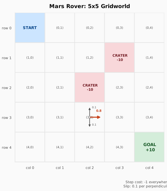
The rules:
- Start: , the top-left corner.
- Goal: , reward , episode ends.
- Craters: and , reward , episode ends.
- Step cost: everywhere else.
- Actions: four moves, encoded as , , , (these are the
[a=…]tags in the trace below). - Slip: the rover moves in the intended direction with probability , and slips to each of the two perpendicular directions (the ones from the intended move) with probability each. Moves into a wall keep the rover in place.
- Discount: .
Let’s build it and watch a random policy fumble around:
import gymnasium as gymfrom gymnasium import spacesimport numpy as npfrom collections import defaultdict
# ══════════════════════════════════════════════════════# Mars Rover Gridworld: a stochastic MDP where the agent must navigate a 5×5# grid to a science target (+10) while avoiding craters (-10).# We build the full environment as a Gymnasium Env so that:#   - DP can read the internal model P[s][a] directly (model-based),#   - MC and TD can only interact via reset()/step() (model-free).# ═══════════════════════════════════════════════════════
# World layout. Coordinates are (row, col), 0-indexed from the top-left corner.# 5x5 board, so 25 discrete states (numbered 0..24)GRID = 5# science target: landing here ends the episode with +10GOAL = (4, 4)# landing in a crater ends the episode with -10CRATERS = {(2, 2), (1, 3)}# probability of slipping to EACH of the two perpendicular tilesSLIP = 0.1# discount: a reward k steps away is worth 0.95**k todayGAMMA = 0.95# action -> (Δrow, Δcol): up, right, down, leftMOVES = {0: (-1, 0), 1: (0, 1), 2: (1, 0), 3: (0, -1)}# perpendicular actions for slip: e.g. "up" can slip to "left" or "right"PERP = {0: [3, 1], 1: [0, 2], 2: [1, 3], 3: [2, 0]}
def rc(s: int) -> tuple[int, int]:    """Given a state index s (0 to GRID*GRID-1), returns (row, col)"""    # divmod(a, b) -> (a // b, a % b)    return divmod(s, GRID)
def idx(r: int, c: int) -> int:    """Given (row, col), returns the flattened state index s"""    return r * GRID + c
class MarsRoverEnv(gym.Env):    def __init__(self):        super().__init__()        # 25 possible states        self.observation_space = spaces.Discrete(GRID * GRID)        # 4 possible moves        self.action_space = spaces.Discrete(4)        self.goal = idx(*GOAL)        self.craters = {idx(*c) for c in CRATERS}        # episode ends in any of these        self.terminals = self.craters | {self.goal}        # full transition model (only DP may read this)        self.P = self._build_model()
    def _move(self, s: int, a: int) -> int:        """Take one step in direction a, clamped so the rover can't walk off the grid. Takes in a state index s and an action index a, and returns the next state index."""        # Find the current row and column of the state        r, c = rc(s)        # Find the delta row and column for the action        dr, dc = MOVES[a]        # Clamp the new row and column to the grid        return idx(min(max(r + dr, 0), GRID - 1), min(max(c + dc, 0), GRID - 1))
    def _reward(self, s_next: int) -> float:        """Reward depends only on which tile you land on. Takes in a next state index s_next, and returns the reward."""        if s_next == self.goal: return 10.0        if s_next in self.craters: return -10.0        # every ordinary step costs 1, which nudges the rover to hurry        return -1.0
    def _build_model(self):        """This block builds the probability distribution over where the rover actually ends up after choosing an action, accounting for slip."""        # This is the "god's-eye" model of the world. DP reads it directly;        # MC and TD are not allowed to, they must learn from reset()/step() only.        # P is a dict, with keys as state indices and values as dictionaries of action indices and lists of tuples (probability, next_state, reward, terminated).        P = defaultdict(dict)        # Iterate over all states        for current_state in range(GRID * GRID):            # For each state s, iterate over all actions a            for action in range(4):                # If the state is a terminal state,                # the rover stays put and earns nothing more.                if current_state in self.terminals:                    P[current_state][action] = [(1.0, current_state, 0.0, True)]                    continue
                # Initialize the outcomes dictionary - maps next_state to its probability                outcomes: dict[int, float] = {}
                # computes the tile the rover wants to reach after taking the action                intended = self._move(current_state, action)
                # It lands there with probability 1 - 2*SLIP                # outcomes.get() -> gives probability of the intended outcome, or 0 if it's not in the dictionary. This accumulates into a dict instead of overwriting.                # This matters because near walls several of these directions can resolve to the same tile (since _move clamps at the edges), and their probabilities must add up rather than clobber each other.                outcomes[intended] = outcomes.get(intended, 0) + (1 - 2 * SLIP)
                # Add the probability of the perpendicular outcomes                # PERP[action] are the two directions perpendicular to the intended one.                # The rover "slips" to each of those with probability SLIP = 0.1 each.                for slip_action in PERP[action]:                    slipped = self._move(current_state, slip_action)                    outcomes[slipped] = outcomes.get(slipped, 0) + SLIP
                # Build the list of transitions for this (current_state, action) pair                transitions = []                for next_state, probability in outcomes.items():                    reward = self._reward(next_state)                    terminated = next_state in self.terminals                    transitions.append((probability, next_state, reward, terminated))                P[current_state][action] = transitions
        return P
    def reset(self, seed=None, options=None):        super().reset(seed=seed)        # every episode begins in the top-left corner        self.s = idx(0, 0)        return self.s, {}
    def step(self, action):        """Simulate a real interaction: sample ONE outcome from P[s][a] according to its probabilities. This is all MC and TD ever see — they never peek at the full distribution, only the single (s', r, terminated) triple that nature dealt."""
        # tr is a list of tuples (probability, next_state, reward, terminated)        transitions = self.P[self.s][action]        # i is the index of the chosen outcome        i = self.np_random.choice(len(transitions), p=[t[0] for t in transitions])        # _ is the probability of the chosen outcome        _, s_next, reward, terminated = transitions[i]        # Update the current state        self.s = s_next        # Return the next state, reward, terminated, truncated, and info        return s_next, reward, terminated, False, {}
# Demonstrate what a policy-less agent looks like: no learning, just random moves.# The rover has no concept of value yet — every direction is equally likely.# This is the "before" picture; DP/MC/TD will give it purposeful behavior.env = MarsRoverEnv()obs, _ = env.reset(seed=42)# reset(seed=...) only seeds the env's internal RNG used by step(); the action# space has its OWN RNG, so we seed it too to make this trace reproducible.env.action_space.seed(42)done = Falsesteps = 0print("Episode trace (random policy):")while not done and steps < 20: # Uniform random action (no intelligence) a = env.action_space.sample() obs_next, r, terminated, truncated, _ = env.step(a) # Show the transition as (row,col) [a=action] → (row,col) and the reward received. # rc(obs) and rc(obs_next) are the row and column of the current and next states print(f" ({rc(obs)[0]},{rc(obs)[1]}) [a={a}] → ({rc(obs_next)[0]},{rc(obs_next)[1]}) r={r:.0f}") obs = obs_next done = terminated or truncated steps += 1if done: print(f" Episode ended at ({rc(obs)[0]},{rc(obs)[1]})")Episode trace (random policy): (0,0) [a=0] → (0,0) r=-1 (0,0) [a=3] → (0,0) r=-1 (0,0) [a=2] → (0,1) r=-1 (0,1) [a=1] → (0,2) r=-1 (0,2) [a=1] → (0,3) r=-1 (0,3) [a=3] → (0,3) r=-1 (0,3) [a=0] → (0,3) r=-1 (0,3) [a=2] → (1,3) r=-10 Episode ended at (1,3)The rover wanders without direction and tumbles into a crater long before it finds the goal. To do better, it needs to know which states are worth being in and which action to take from each one. That’s exactly what DP, MC, and TD compute, each from a different kind of information.
Before moving on, let’s peek at the transition model we just built. env.P[s][a] lists every (probability, next_state, reward, terminated) the rover could face. Two cases are worth seeing: an open cell, and a cell against a wall.
# P[s][a] is a list of (probability, next_state, reward, terminated).# Print where each action could land the rover, and with what probability.def show(state, action, label):    print(f"{label}: from {rc(state)} taking a={action}")    for p, s_next, r, terminated in env.P[state][action]:        print(f"    p={p:.1f} → {rc(s_next)}  r={r:.0f}")
# Open cell: the three outcomes are three distinct tiles -> a clean 0.8 / 0.1 / 0.1.show(idx(1, 1), 0, "Open space") # 'up' from (1,1)# Wall cell: 'up' is clamped back onto the same tile, so probabilities MERGE.show(idx(0, 0), 0, "Corner (wall)") # 'up' from (0,0)Open space: from (1, 1) taking a=0 p=0.8 → (0, 1) r=-1 p=0.1 → (1, 0) r=-1 p=0.1 → (1, 2) r=-1Corner (wall): from (0, 0) taking a=0 p=0.9 → (0, 0) r=-1 p=0.1 → (0, 1) r=-1In open space you get the textbook split: 80% to the intended tile, 10% to each perpendicular. Against the top wall, “up” (0.8) and the leftward slip (0.1) both clamp back onto (0,0), so their probabilities add to 0.9. This is why _build_model accumulates with outcomes.get(next_state, 0) + p instead of overwriting: whenever wall-clamping sends several directions to the same tile, their mass must pool so each row still sums to 1.
Here’s the grid once more, so you can read the traces above against the map without scrolling back up:
The video-game-level analogy
Imagine a 4-stage video game level with a randomized boss at stage 3:
- DP reads the game’s source code (the model). It computes the exact expected score from every checkpoint without playing once.
- MC plays the level start-to-finish many times, records the total score from each run, and averages them per checkpoint.
- TD plays the level but updates its estimate of each checkpoint after every single stage transition, using its current (imperfect) estimate of the next stage.
Same question, same answer, three routes to get there.
2. The math you need
2.1 Value Iteration (Dynamic Programming)
DP uses the full model to sweep the Bellman optimality equation across every state:
Each sweep applies this backup to every state. After enough sweeps, converges to .
Why does it converge? The Bellman operator is a contraction mapping: each application brings closer to by a factor of . Think of a photocopier set to 95% zoom: no matter what you start with, repeated copies shrink toward a dot. After sweeps:
Let’s read that term by term:
- is your value estimate after sweeps; is the true optimal value we’re chasing.
- is the worst error across all states. The subscript is the max-norm: compute the absolute gap at every state , then keep the single largest one. So if this number is small, every state is close, not just the average state.
- The inequality says that worst error is at most times the error you began with (). Each sweep multiplies your remaining error by a factor of at most , so it shrinks geometrically:
Because , that bound is guaranteed to reach 0 no matter how wrong your starting guess was. That is exactly what “contraction” means: the Bellman backup always pulls any value estimate closer to , so there’s a single fixed point everything funnels into. Your starting guess only affects how many sweeps you need, never whether you arrive.
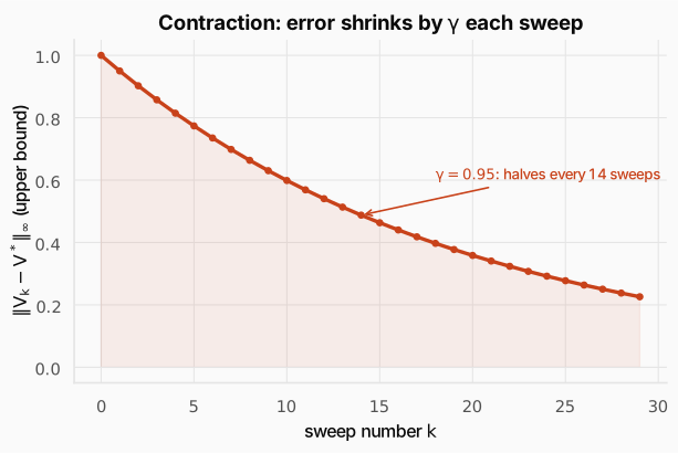
The figure plots that upper bound against the sweep number . It starts at (at sweep you could be 100% of your initial error off) and decays smoothly toward , the shaded area underneath showing the error budget vanishing. With the decay is gentle: the marked point shows the error halving roughly every 14 sweeps. A smaller (a more myopic agent) would plunge to zero much faster, while a near flattens the curve and needs more sweeps. Either way, convergence to the exact answer is guaranteed.
def value_iteration(env, gamma=GAMMA, theta=1e-6):    """Bellman optimality backup: V(s) ← max_a Σ p(s'|s,a)[r + γ·V(s')]    Sweeps all states repeatedly until values stop changing (< theta)."""    # start every state's value at 0 (arbitrary guess)    V = np.zeros(env.observation_space.n)    while True:        # Track largest change this sweep for convergence check        delta = 0        for s in range(env.observation_space.n):            v_old = V[s]            q_values = []            for a in range(env.action_space.n):                # Q(s,a) = Σ p · [r + γ·V(s')·(1-done)]                # The (1-done) factor ensures terminal states contribute 0 future value,                # because once the episode ends there's nothing more to collect.                q = 0                for probability, s_next, r, done in env.P[s][a]:                    q += probability * (r + gamma * V[s_next] * (1 - done))                # Add the Q-value for this action to the list                q_values.append(q)
            # Bellman optimality: the value of a state under the BEST policy is the max over actions            V[s] = max(q_values)            # Track the change for convergence check            delta = max(delta, abs(v_old - V[s]))        # Convergence: when the biggest value change in a full sweep is negligible,        # we've found V* (guaranteed by the contraction mapping theorem).        if delta < theta:            break
    # Extract the greedy policy: π*(s) = argmax_a Q(s,a).    # Given the optimal values, the best action is the one with the highest expected return.    policy = np.zeros(env.observation_space.n, dtype=int)    for s in range(env.observation_space.n):        q_values = []        for a in range(env.action_space.n):            q = 0.0            for p, s_next, r, done in env.P[s][a]:                q += p * (r + gamma * V[s_next] * (1 - done))            q_values.append(q)        policy[s] = np.argmax(q_values)    return V, policy
env = MarsRoverEnv()V_dp, policy = value_iteration(env)
# Display V* as a 5×5 grid — higher values mean "closer to the goal in expectation"print("V* (5x5 grid):")print(V_dp.reshape(5, 5).round(2))
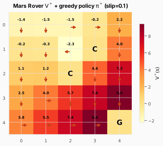
# Show the optimal policy as directional arrows# This is what a perfectly rational rover would do at each cellprint("\nGreedy policy (^>v<):")arrows = {0: "^", 1: ">", 2: "v", 3: "<"}grid = []for s in range(25): grid.append("." if s in env.terminals else arrows[policy[s]])print(np.array(grid).reshape(5, 5))V* (5x5 grid):[[-1.42 -1.5 -1.52 -0.21 2.24] [-0.18 -0.29 -2.26 0. 4.02] [ 1.13 1.25 0. 4.56 7.28] [ 2.51 4. 5.73 7.59 9.42] [ 3.8 5.53 7.4 9.42 0. ]]
Greedy policy (^>v<):[['v' 'v' '>' '>' 'v'] ['v' 'v' '<' '.' 'v'] ['v' 'v' '.' 'v' 'v'] ['v' '>' 'v' 'v' 'v'] ['>' '>' '>' '>' '.']]Values increase as you approach the goal. The policy steers down and right toward (4,4), but detours around craters: cell (1,2) goes left to avoid both the crater at (1,3) and (2,2).
What if terrain were perfect?
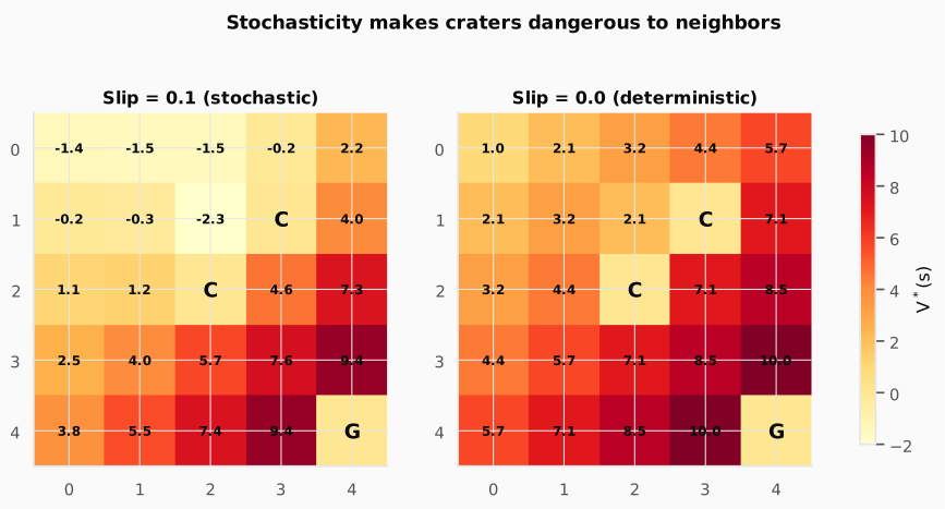
With SLIP=0, the rover has perfect control. Craters only hurt if you deliberately enter them:
# Experiment: what happens if we remove stochasticity entirely?# With SLIP=0 the rover always goes exactly where it intends — no random drift# into craters. This isolates how much of the danger comes from slip vs. proximity.SLIP = 0.0env_det = MarsRoverEnv()V_det, _ = value_iteration(env_det)SLIP = 0.1 # restore stochastic terrain for subsequent experimentsprint("V* with SLIP=0 (deterministic):")# Compare this to the stochastic grid: crater-adjacent cells should now be positive# because the rover can simply avoid stepping into them.print(V_det.reshape(5, 5).round(2))V* with SLIP=0 (deterministic):[[ 0.95 2.05 3.21 4.44 5.72] [ 2.05 3.21 2.05 0. 7.07] [ 3.21 4.44 0. 7.07 8.5 ] [ 4.44 5.72 7.07 8.5 10. ] [ 5.72 7.07 8.5 10. 0. ]]Without slip, crater-adjacent cells have positive values: they’re safe if you never step in voluntarily. Stochasticity is what makes craters dangerous to neighbors, not the craters themselves.
Check: Why is value iteration guaranteed to converge? What property of the Bellman operator forces it?
Answer. Because the Bellman operator is a -contraction in the sup-norm: one backup moves any two value estimates strictly closer, by at least a factor (that is ). The Banach fixed-point theorem then forces a unique fixed point () and geometric convergence to it from any starting guess.
Check: Set `SLIP` from 0.1 to 0 (perfect terrain) and re-run. What changes in the values near the craters, and why?
Answer. With perfect control the crater-adjacent cells flip to positive values: they are only dangerous if you deliberately step in. Under slip, a neighboring cell carries a real chance of being thrown into the crater, so its value drops. The craters never changed; stochasticity is what makes them dangerous to their neighbors.
Value iteration is one DP route, but not the only one. The classic alternative, policy iteration, splits the work in two: fully evaluate a fixed policy (Bellman expectation sweeps from MDPs & Bellman until its values settle), then improve it greedily with , and repeat. On a 25-state grid both land on the same , so we won’t re-derive it here. The part worth remembering is the pattern: this evaluate ↔ improve loop, generalized policy iteration, is the skeleton that Monte Carlo and TD control will reuse once we drop the model.
One setup detail before MC and TD. The next two methods do prediction: they estimate for a given policy , so they each need a policy handed to them. We deliberately reuse the optimal policy that DP just computed. Why? So all three methods estimate the same target. DP gives us exactly; MC and TD then try to reach those same numbers from sampled experience alone. That makes the comparison apples-to-apples and turns DP’s output into a ground-truth answer key we can check MC and TD against. (MC and TD don’t need DP, they can evaluate any policy with no model; we just borrow so “same value, three different ways” is verifiable.)
2.2 Monte Carlo Prediction
MC doesn’t need the model, only the ability to play episodes. Run the policy, record what happens, and average the realized returns:
where is the actual discounted return from state onward.
Properties:
- Unbiased: is the true return, not an approximation.
- High variance: one unlucky episode can wildly swing the estimate.
- Must wait until episode end to compute .
def mc_prediction(env, policy, episodes=20000, gamma=GAMMA, alpha=0.02, max_steps=100):    """Monte Carlo prediction: estimate V^π by playing full episodes and averaging    the actual discounted returns observed from each state. No model needed —    only the ability to run reset()/step()."""    V = np.zeros(env.observation_space.n)    for _ in range(episodes):        # Phase 1: Generate a complete episode trajectory under the given policy.        # We store (state, reward) pairs to compute returns afterward.        episode = []        s, _ = env.reset()        for _ in range(max_steps):            # follow the fixed policy we are evaluating            a = policy[s]            s_next, reward, terminated, truncated, _ = env.step(a)            episode.append((s, reward))            s = s_next            if terminated or truncated:                break        # Phase 2: Compute returns backward. Starting from the final step,        # accumulate G_t = r_{t+1} + γ·G_{t+1}. This is the TRUE discounted sum        # of rewards from that state onward — unbiased but high-variance.        G = 0.0        for s, reward in reversed(episode):            # G_t = r + γ·G_{t+1} (the recursive return)            G = reward + gamma * G            # Incremental mean update: nudge V(s) toward this episode's return G.            # α controls the step size — too large = noisy, too small = slow learning.            # MC update: V(s) ← V(s) + α·[G_t - V(s)]            V[s] = V[s] + alpha * (G - V[s])    return V
env = MarsRoverEnv()_, policy = value_iteration(env)# Show convergence progress: MC gets noisier estimates with fewer episodesfor n in [1000, 5000, 20000]: V_mc = mc_prediction(env, policy, episodes=n) print(f"MC after {n:,} episodes: V(start)={V_mc[0]:.2f}")print(f"\nMC final grid (20k episodes):")print(V_mc.reshape(5, 5).round(2))MC after 1,000 episodes: V(start)=-1.49MC after 5,000 episodes: V(start)=-1.19MC after 20,000 episodes: V(start)=-1.43
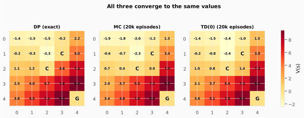
MC final grid (20k episodes):[[-1.43 -1.33 -0.49 0.55 2.94] [-0.41 -0.42 -2.59 0. 4.77] [ 0.99 0.83 0. 1.58 7.77] [ 2.28 3.7 5.97 7.79 9.55] [ 3.7 5.01 7.45 9.46 0. ]]The MC estimates are close to the DP values but still noisy: fluctuates because the start state is far from the goal, giving high-variance returns.
2.3 TD(0) Prediction: The Breakthrough
TD doesn’t wait for the episode to end. After each step, it updates using the observed reward plus the estimated value of the next state:
The term is the TD error: “how much more (or less) I got than I expected.” If my estimate was perfect, .
Remember the running average from RL intro & prerequisites? This update isn’t new, it’s that exact rule. Blog 1 called “the template for every learning rule in RL,” and TD(0) is that template with the pieces renamed:
So the TD error is just the error term from blog 1, “how far the target is from what I currently believe,” and we step a fraction of the way toward it. The only thing that changes between methods is what plays the role of the target :
- Monte Carlo: , the actual, fully-observed return. You wait for the episode to end, then average toward a real sample (exactly the law-of-large-numbers averaging from blog 1).
- TD(0): , a bootstrapped target, one real reward plus your current estimate of the rest. No waiting required.
That single substitution is the entire difference between MC and TD. It’s also why when your estimate is already self-consistent: the target equals the current value, so there’s nothing left to nudge.
Properties:
- Biased early: it bootstraps off , which starts wrong.
- Low variance: uses a single transition, not an entire episode’s worth of randomness.
- Updates every step: no need to wait for episode end; works for continuing tasks too.
def td_prediction(env, policy, episodes=20000, gamma=GAMMA, alpha=0.05, max_steps=100):    """TD(0) prediction: estimate V^π by bootstrapping — after each single step,    update V(s) toward (r + γ·V(s')), using our CURRENT estimate of the next state    as a stand-in for the true future return. No full episodes needed."""    V = np.zeros(env.observation_space.n)    for _ in range(episodes):        s, _ = env.reset()        for _ in range(max_steps):            # follow the fixed policy we are evaluating            a = policy[s]            s_next, reward, terminated, truncated, _ = env.step(a)            # Bootstrap: V(s') is our current (imperfect) estimate of future value.            # At a terminal state, there IS no future, so bootstrap = 0.            bootstrap = V[s_next] if not terminated else 0.0            # TD target = r + γ·V(s'): one real reward + discounted estimate of the rest.            # TD error δ = target - V(s): how much better/worse reality was than predicted.            td_error = reward + gamma * bootstrap - V[s]            # TD(0) update: V(s) ← V(s) + α·δ — nudge value by a fraction of the surprise.            # Unlike MC, this fires EVERY step, so information propagates much faster.            V[s] = V[s] + alpha * td_error            s = s_next            if terminated or truncated:                break    return V
env = MarsRoverEnv()_, policy = value_iteration(env)# Show convergence progress: TD updates at every step, so it often converges# faster than MC even with the same number of episodes.for n in [1000, 5000, 20000]: V_td = td_prediction(env, policy, episodes=n) print(f"TD(0) after {n:,} episodes: V(start)={V_td[0]:.2f}")print(f"\nTD(0) final grid (20k episodes):")print(V_td.reshape(5, 5).round(2))TD(0) after 1,000 episodes: V(start)=-1.15TD(0) after 5,000 episodes: V(start)=-1.38TD(0) after 20,000 episodes: V(start)=-1.42
TD(0) final grid (20k episodes):[[-1.42 -1.69 -1.57 0.15 2.48] [-0.24 -0.21 -2.13 0. 4.5 ] [ 1.32 0.98 0. 3.26 7.29] [ 2.59 3.74 5.76 7.48 8.95] [ 3.81 5.36 7.72 9.26 0. ]]TD converges closer to the DP answer with less noise: it updates 25 states per episode (one per step) versus MC’s single batch at the end.
Check: Define bootstrapping in one sentence. Then explain why it is simultaneously the source of TD's speed and the source of its instability.
Answer. Bootstrapping means updating an estimate using other current estimates instead of waiting for the true return. It is the source of TD’s speed because you can update every single step without finishing the episode. It is also the source of its instability because errors in those estimates feed straight back into the targets, and with function approximation they can amplify (the deadly triad, which we hit in SARSA, Q-learning & DQN).
Check: You hit a crater on episode 1. With MC, when does the state just before it learn it was bad? With TD?
Answer. With MC, only at the end of the episode: the preceding state’s value waits for the full return , which doesn’t exist until the run is over. With TD, immediately on that step: the enters for the transition into the crater, so the state before it is corrected one step later instead of one episode later.
Check: The TD target r + gamma V(s') is a "proxy" for the true return G. It is an approximation because V(s') starts wrong. So why does repeatedly using this noisy proxy converge to the correct values?
Answer. Because the proxy is grounded in the Bellman equation: if were correct, would equal the true expected return exactly. Each update nudges a fraction toward that proxy, and as improves, the proxy improves too. The errors shrink in a virtuous circle, and under standard conditions (enough visits, a decaying step size) the process converges to the unique fixed point of the Bellman equation, the true value function.
2.4 The DP / MC / TD Tradeoff
| Property | DP | MC | TD |
|---|---|---|---|
| Needs model | yes | no | no |
| Bootstraps from | yes | no | yes |
| Updates use sampled outcome | no, exact expectation | yes, full-episode return | yes, one transition |
| When does the update fire? | every sweep, every state | end of episode only | after every step |
| Variance | none (deterministic) | high (whole-episode return) | moderate (one-step) |
| Bias | none at convergence | none at convergence | nonzero while is learning |
All three converge to the same , and here’s the proof:
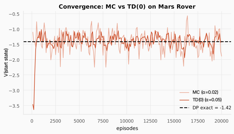
And here they are side by side as heatmaps:
Check: You're handed a brand-new environment with no model of its dynamics. Of DP, MC, and TD, which are even available to you, and why is one ruled out?
Answer. Only MC and TD. Both learn straight from sampled reset()/step() experience. DP is ruled out because its backup needs the full model and the reward function up front, which a brand-new environment doesn’t hand you. This is exactly why the rover env exposes P for DP while the model-free methods never touch it (and why MC/TD are the realistic choice for a real Mars rover).
Check: MC and TD both converge to the same values, so why does TD typically get there in far fewer episodes? What is it exploiting that MC throws away?
Answer. TD bootstraps: it reuses its current estimate of the next state’s value immediately, so a reward’s information propagates after a single transition. MC discards that intermediate structure and waits for the whole-episode return, so every update is one noisy full-episode sample, carrying far less information per step. Same destination, fewer episodes.
Check: Name one situation where you'd actually prefer Monte Carlo over TD.
Answer. When episodes are short and cheap and you want zero bootstrap bias, or early in training when the value estimates are still unreliable so bootstrapping would inject bad bias. MC is unbiased; when variance isn’t the bottleneck, that can win.
2.5 Prediction vs Control: The Bridge to Q-Learning
Everything so far has been prediction: someone hands you a policy , and you answer one question, “how good is it?”, by estimating . DP, MC, and TD all chased that same number, just from different information. Notice what prediction never does: it never changes how the rover behaves. The policy is frozen; we only score it.
But scoring a fixed policy was never the real goal. What we actually want is control: not “how good is this policy?” but “what is the best policy?”, the one that earns the most return from every state.
So why not just reuse a tool we already have? Each one hits a wall.
DP can do control, but only with a model. Value iteration already found through its step, so DP is a control method. The catch is what it demands: the full transition model and a sweep over every state on every iteration. We had both for a 25-cell grid, but real problems usually offer neither, no god’s-eye model of the world, and far too many states (often continuous) to enumerate. DP control is exact only when you can afford to read and iterate the entire model, which is almost never.
Pure MC and TD predict, but can’t improve as described. Estimating from samples removes the model requirement, which fixes DP’s first problem, but two gaps remain. First, alone can’t tell you which action to take: turning a state value into a greedy choice means looking one step ahead with , the very model we just said we don’t have. Second, they only ever follow the fixed policy , so they only see the actions already takes and never gather evidence about the alternatives you’d need in order to improve.
The fix closes both gaps at once: learn for every action (not just the one the policy takes), so the best action is a direct lookup with no model needed, and keep exploring so those alternative actions actually get visited. Then pick the best:
That leap (TD + Q-values + ) is Q-learning, the subject of SARSA, Q-learning & DQN. Every modern algorithm (DQN, PPO, GRPO) traces back to this one-step TD update scaled up.
Check: Next we replace the value table with a neural network. Which term in the TD update R + γV(s′) − V(s) becomes the "loss" we minimize?
Answer. The TD error itself, . We turn the target into a regression label and minimize the squared TD error. That squared error is precisely the DQN loss in the next post.
Check: A chess player who never improves still has a value function. What does "prediction" (evaluate) mean for that player, and how does "control" go one step further?
Answer. Prediction asks: “given this player’s fixed, possibly terrible style, what is the expected outcome from each board position?” The policy stays frozen; we just score it. Control asks: “can we improve the style itself?” It checks whether any action beats the current value, updates the policy, re-evaluates, and repeats. Prediction tells you how good your habits are; control changes them.
2.6 Putting it all together: All three on Mars Rover
| Concept | Math | In code |
|---|---|---|
| Bellman optimality backup | V[s] = max(q_values) | |
| MC return | G = reward + gamma * G | |
| MC update | V[s] += alpha * (G - V[s]) | |
| TD target | reward + gamma * V[s_next] | |
| TD update | V[s] += alpha * (target - V[s]) |
Practice: assignment
Put all three methods to work — build a Mars Rover environment, solve it with Value Iteration (DP), then estimate the same values with Monte Carlo and TD(0) and watch them converge:
Where this goes next
We’ve solved prediction (estimating for a given policy) three ways. But the real goal is control: finding the best policy without being handed one.
The trick: replace with , apply the TD update to every state-action pair, and use to learn the optimal policy while exploring:
That’s Q-learning, the algorithm that launched Deep RL when combined with a neural network (DQN). The SARSA, Q-learning & DQN post builds it from scratch.